自己建网站难吗拉新平台
目录
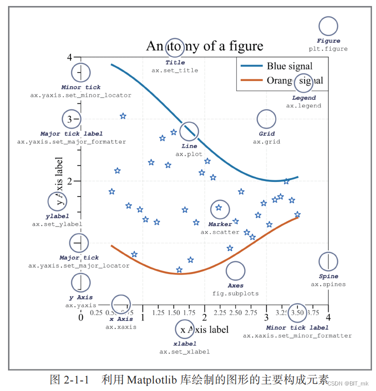
图形元素
画布 (fifigure)。
坐标图形 (axes),也称为子图。
轴 (axis) :数据轴对象,即坐标轴线。
刻度 (tick),即刻度对象。
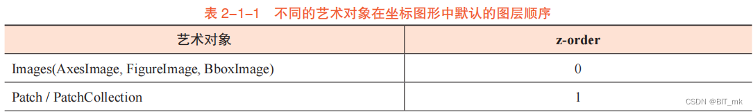
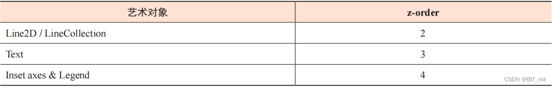
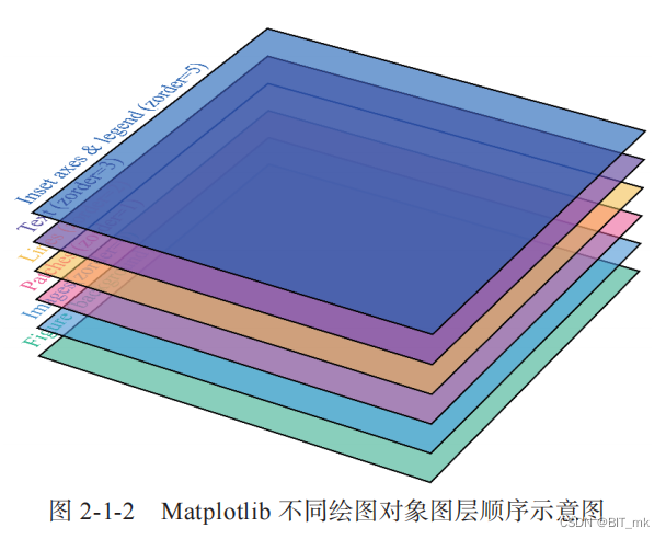
图层顺序
轴比例和刻度
轴比例
刻度位置和刻度格式
坐标系
直角坐标系
极坐标系
地理坐标系
多子图的绘制
subplot() 函数
add_subplot() 函数
subplots() 函数
axes()
subplot2grid() 函数
gridspec.GridSpec() 函数
subplot_mosaic() 函数
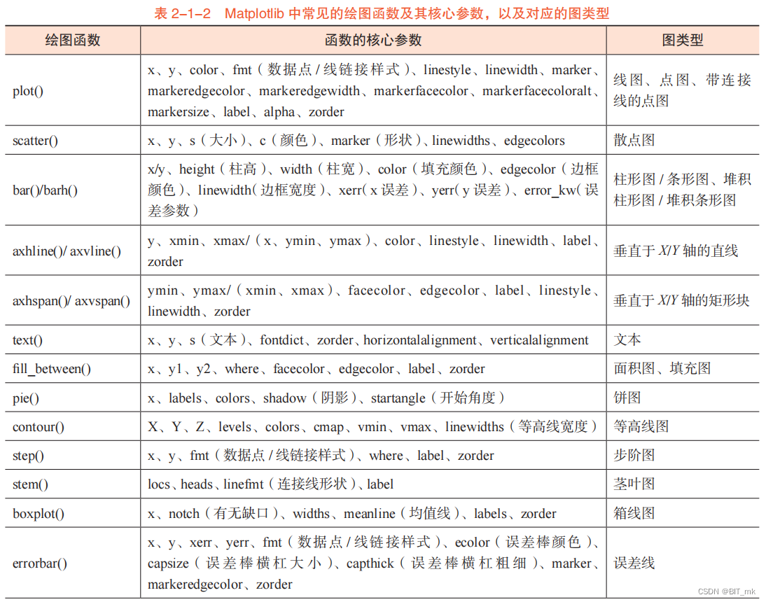
常见的图的类型
结果保存
图形元素
-
画布 (fifigure)。
它既可以代表图形本身进行图的绘制(包含图例、图名、数据标记等多个图形艺术对象,又可以 被划分为多个子区域,而每个子区域可用于单独图形类型的 ( 子图 ) 绘制。用户可以在画布 (fifigure) 中设置画布大小(fifigsize)、分辨率(dpi)和背景颜色等其他参数。
-
坐标图形 (axes),也称为子图。
作为 Matplotlib 的绘图核心,它主要为绘图数据提供展示区域,同时包括组成图的众多艺术对象 (artist)。在大多数情况下,一个画布 (fifigure) 对象中包含一个子图区域,子图区域由上、下、左、右 4 个轴脊以及其他构成子图的组成元素组成。
-
轴 (axis) :数据轴对象,即坐标轴线。
每个轴对象都含有位置( locator )对象和格式(formatter )对象,它们分别用于控制坐标轴刻度的位置和格式。
-
刻度 (tick),即刻度对象。
刻度对象包括主刻度(Major tick)、次刻度(Minor tick)、主刻度标签(Major tick label)和次刻度标签(Minor tick label)。
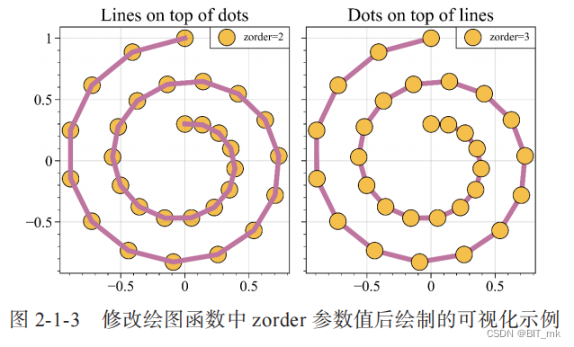
图层顺序
Matplotlib 采用的是面向对象的绘图方式。在同一个坐标图形中绘制不同的数据图层时,
Matplotlib 可通过设置每个绘图函数中的 zorder 参数来设定不同的图层。
轴比例和刻度
Matplotlib 中 的每个坐标图形对象至少包含两个轴对象,它们分别用来表示 X 轴和 Y 轴。轴对象还可以控制轴比例(axis scale )、刻度位置( tick locator )和刻度格式( tick formatter )。
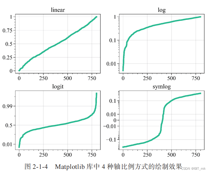
轴比例
轴比例规定了数值与给定轴之间的映射方式,即数值在轴上以何种方式进行缩放。Matplotlib 中的默认轴比例方式为线性( linear )方式,其他诸如 log 、 logit 、 symlog 和自定义函数比例(function scale )方式也是常用的轴比例方式。
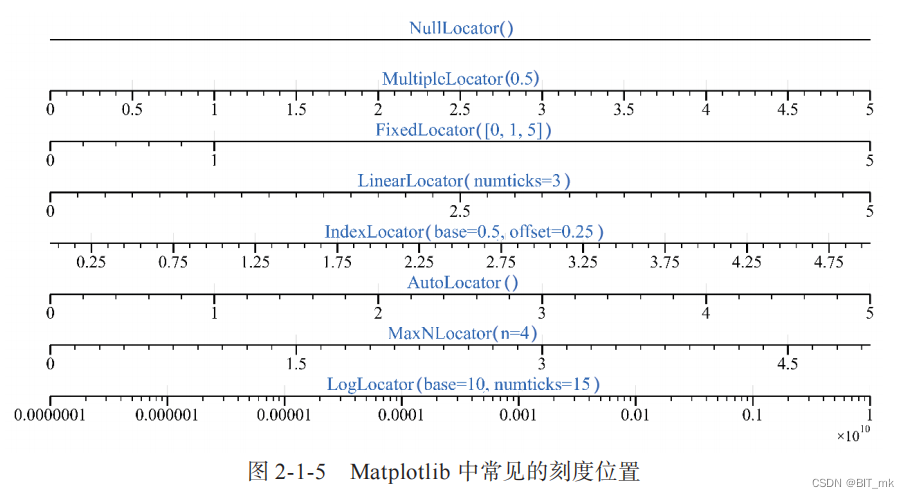
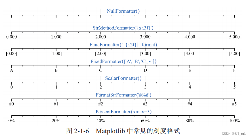
刻度位置和刻度格式
刻度位置和刻度格式分别规定了每个轴对象上刻度的位置与格式。
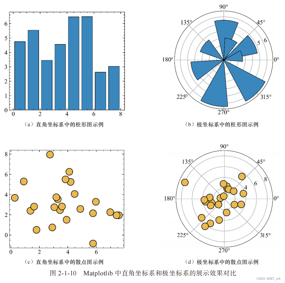
坐标系
常见的坐标系有直角坐标系( rectangular coordinate system )、极坐标系( polar coordinate
system )和地理坐标系( geographic coordinate system )。
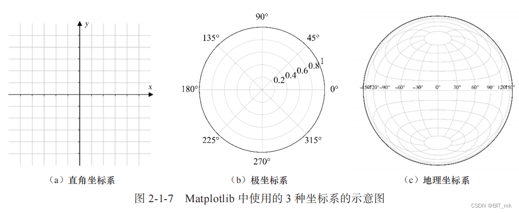
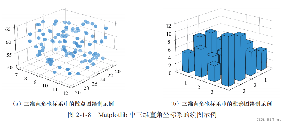
直角坐标系
Matplotlib 中,我们可通过设置绘图函数(如 add_subplot() )中的参数 projection='3d' 或引入 axes3d 对象来绘制三维直角坐标系。
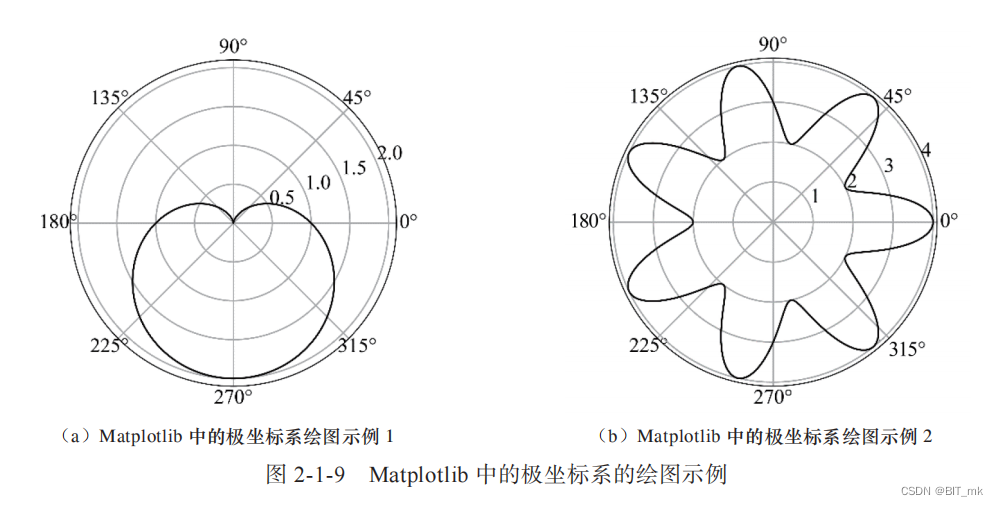
极坐标系
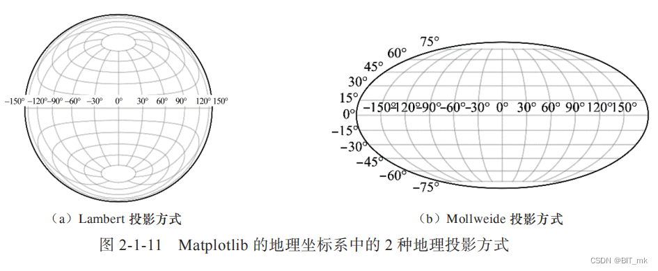
地理坐标系
Matplotlib 地理坐标系中的地理投影方式较少,仅有 Aitoffff 投影、 Hammer 投影、 Lambert
投影和 Mollweide 投影 4 种。
多子图的绘制
subplot() 函数
import matplotlib.pyplot as plt
ax1 = plt.subplot(212)
ax2 = plt.subplot(221)
ax3 = plt.subplot(222)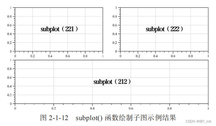
add_subplot() 函数
import matplotlib.pyplot as plt
fig = plt.figure()
ax1 = fig.add_subplot(212)
ax2 = fig.add_subplot(221)
ax3 = fig.add_subplot(222)
subplots() 函数
fig, axs = plt.subplots(2, 3, sharex=True, sharey=True)
axs[0,0].text(0.5, 0.5, "subplots(0,0)")
axs[0,1].text(0.5, 0.5, "subplots(0,1)")
axs[0,2].text(0.5, 0.5, "subplots(0,2)")
axs[1,0].text(0.5, 0.5, "subplots(1,0)")
axs[1,1].text(0.5, 0.5, "subplots(1,1)")
axs[1,2].text(0.5, 0.5, "subplots(1,2)")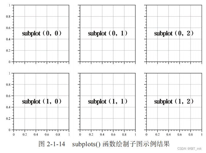
axes()
import numpy as np
import matplotlib.pyplot as plt
from colormaps import parula
np.random.seed(19680801)
plt.subplot(211)
plt.imshow(np.random.random((100, 100)),cmap=parula)
plt.subplot(212)
plt.imshow(np.random.random((100, 100)),cmap=parula)
plt.subplots_adjust(bottom=0.1, right=0.8, top=0.9)
cax = plt.axes(rect=[0.8, 0.15, 0.05, 0.6])
plt.colorbar(cax=cax)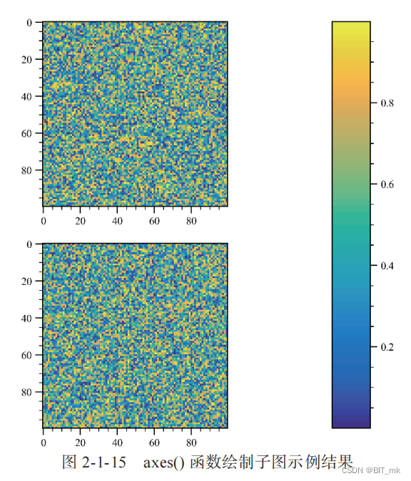
subplot2grid() 函数
import matplotlib.pyplot as plt
fig = plt.figure()
ax1 = plt.subplot2grid((3, 3), (0, 0), colspan=3)
ax2 = plt.subplot2grid((3, 3), (1, 0), colspan=2)
ax3 = plt.subplot2grid((3, 3), (1, 2), rowspan=2)
ax4 = plt.subplot2grid((3, 3), (2, 0))
ax5 = plt.subplot2grid((3, 3), (2, 1))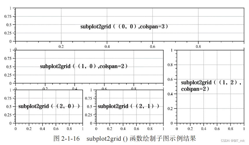
gridspec.GridSpec() 函数
import matplotlib.pyplot as plt
import matplotlib.gridspec as gridspec
fig = plt.figure(constrained_layout=True)
gspec = gridspec.GridSpec(ncols=3, nrows=3, figure=fig)
ax1=plt.subplot(gspec[0,:])
ax2=plt.subplot(gspec[1,0:2])
ax3=plt.subplot(gspec[1:,2])
ax4=plt.subplot(gspec[2,0])
ax5=plt.subplot(gspec[-1,-2])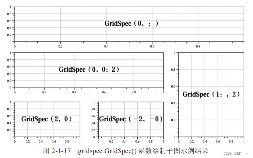
subplot_mosaic() 函数
def annotate_axes(ax, text, fontsize=fontsize):ax.text(0.5, 0.5, text, transform=ax.transAxes,fontsize=fontsize, alpha=0.75, ha="center",va="center", weight="bold")
fig, axd = plt.subplot_mosaic([['upper left', 'right'],['lower left', 'right']],figsize=(6,3), constrained_layout=True)
for k in axd:annotate_axes(axd[k], f'axd["{k}"]', fontsize=14)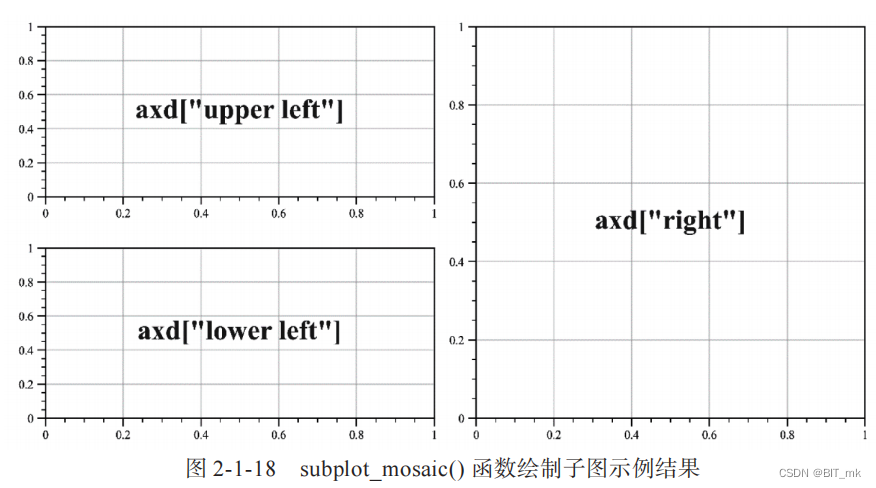
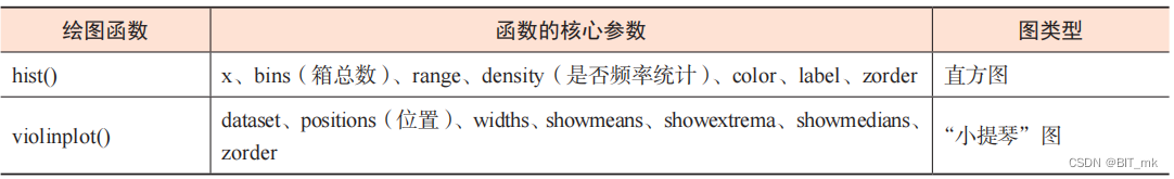
常见的图的类型
结果保存
Matplotlib 绘制的图对象可以保存为多种格式,如 PNG 、 JPG 、 TIFF 、 PDF 和 SVG 等。注意,结果保存函数 savefifig() 必须出现在 show() 函数之前,可避免保存结果为空白等问题。另外,在使用 savefifig() 的过程中,我们需要设置参数 bbox_inches='tight' ,去除图表周围的空白部分。将图对象保存为 PDF 文件和 PNG 文件的示例代码如下。
fig.savefig('结果.pdf',bbox_inches='tight')
fig.savefig('结果.png', bbox_inches='tight',dpi=300)
plt.show()